Let's say you are building a predictive model based on a data set that has well over 100+ columns (aka features), should you use all of them? The short answer is 'no'. Having too many features potentially adds redundancy, reduces model accuracy and over complicates (think of 'Occam's Razor').
So how do you select the fewest and best predictors in your data set to build your machine learning model?

Enter Boruta (and no I'm not referring to the forest demon god known in Slavic mythology). I'm referring to the Boruta package in R that was first published in 2010. I have found great success for reducing the number of dependent variables and selecting only the top predictors (aka feature selection) for my machine learning building efforts. For those interested in applying this in R, Analytics Vidhya has a great example to reference.
I'll admit, I'm an R guy and still remain so; however, in order for me to "play nice" with other data scientists I find myself more and more these days replicating what I already know in R into Python, which isn't always an easy feat. This is especially true when I know I can complete the same thing in half the time or less in R versus Python. But hey, that's how we all get better and expand our skills by pushing ourselves, right?
As a result, the purpose of this blog is to share my attempt in replicating Boruta in Python, which I was recently able to do so after coming across Samuele Mazzanti's well written article titled "Boruta Explained Exactly How You Wished Someone Explained to You". I highly encourage to read his article for anyone looking to learn more. Below is my personal attempt to replicating Boruta in Python after reading this. To view the entire code for this project, feel free to follow along by viewing my repository on GitHub.
Getting started in Python
Let’s first build a small data set with 3 features (age, height and weight), a target variable (income) and 5 observations. This obviously is not a real world example, but gives us something to work with for our purposes.
The goal is to predict income of a person knowing his/her age, height and weight but automatically selecting the best predictive features.
import pandas as pd

X = pd.DataFrame(
{'age': [25,32,47,51,62],
'height': [182, 176, 174, 168, 181],
'weight': [75, 71, 78, 72, 86]})

y = pd.Series([20, 32, 45, 55, 61], name = 'income')
After creating the data above, the following is my attempt to replicate Boruta in Python using Mazzanti's article as previously mentioned. I have applied Boruta for feature selection in many instances in R, but this is my first attempt in Python.
How to replicate Boruta in Python?
A popular algorithm for feature selection is sklearn’s SelectFromModel. Basically, you choose a model of convenience - capable of capturing non-linear relationships and interactions, e.g. a random forest - and you fit it on X and y. Then you extract the importance of each feature from this model and keep only the features that are above a given threshold of importance.
This sounds reasonable, but who determines the threshold, and how?
Enter Boruta. Boruta uses a feature selection algorithm that is statistically grounded and works extremely well even without any specific input by the user. How is this even possible?
Boruta is based on two brilliant ideas.
Idea #1: Shadow Features
In Boruta, features do not compete among themselves. Instead - and this is the idea - they compete with a randomized version of them.
In practice, starting from X, another dataframe is created by randomly shuffling each feature. These permuted features are called shadow features. A this point, the shadow dataframe is attached to the original dataframe to obtain a new dataframe (we will call it X_boruta), which has twice the number of columns of X.
import numpy as np

### make X_shadow by randomly permutating each column of X
np.random.seed(42)
X_shadow = X.apply(np.random.permutation)
X_shadow.columns = ['shadow_' + feat for feat in X.columns]
print(X_shadow)

   shadow_age  shadow_height  shadow_weight
0          51            176             75
1          32            182             71
2          47            168             78
3          25            181             72
4          62            174             86

### make X_boruta by appending X_shadow to X
X_boruta = pd.concat([X,X_shadow], axis = 1)
print("\n\n", X_boruta)

   age  height  weight  shadow_age  shadow_height  shadow_weight
0   25     182      75          51            176             75
1   32     176      71          32            182             71
2   47     174      78          47            168             78
3   51     168      72          25            181             72
4   62     181      86          62            174             86
Then, a random forest is fitted on X_boruta and y.
Now, we take the importance of each original features and compare it with the a threshold. This time, the threshold is defined as the highest feature importance recorded among the shadow features. When the importance of a feature is higher than this threashold, this is called a "hit". The idea is that a feature is usefule only if it's capable of doing better than the best randomized feature.
The code to reproduce this process is the following:
from sklearn.ensemble import RandomForestRegressor
from matplotlib import pyplot

### fit a rf (suggested max_depth between 3 and 7)
forest = RandomForestRegressor(max_depth = 5, random_state = 42, n_estimators=100)
forest.fit(X_boruta, y)

print(X.columns)
>['age', 'height', 'weight']

### store feature importances
feat_imp_X = forest.feature_importances_[:len(X.columns)]
print("\n Feature VIM = ", feat_imp_X,"\n")
> Feature VIM =  [0.39036271 0.19456196 0.07606017]

feat_imp_shadow = forest.feature_importances_[len(X.columns) :]
print("\n Shadows VIM = ", feat_imp_shadow,"\n")
> Shadows VIM =  [0.11033247 0.14261304 0.08606966]

### compute Shadow Threshold & Hits
print("\n Shadow Threshold = ", round(feat_imp_shadow.max(),3),"\n")
> Shadow Threshold =  0.143

hits = feat_imp_X > feat_imp_shadow.max()
print("\n Hits = ", hits, "\n")
> Hits =  [ True  True False]

# get importance
importance = forest.feature_importances_
importance_df = pd.DataFrame({'feature': X_boruta.columns,'vim': importance})

# summarize feature importance
for index,row in importance_df.iterrows():
    print( 'Feature: ', row['feature'], ', Score: ', round(row['vim'],3))

> Feature:  age , Score:  0.39
> Feature:  height , Score:  0.195
> Feature:  weight , Score:  0.076
> Feature:  shadow_age , Score:  0.11
> Feature:  shadow_height , Score:  0.143
> Feature:  shadow_weight , Score:  0.086
Based on the outputs above, we can determine that the shadow threshold is 14.3%, thus 2 features made the hit, namely age and height (39% and 19.5%, respectively), whereas weight (8.6%) scored below the threshold.
Apparently, we should drop weight and get on with age and *height. BUT should we trust this run? What if it was just an unlucky run for weight? What if instead it was just a lucky run for age and height?
This is where the second brilliant idea of Boruta comes into play.
Idea #2: Binomial Distribution
As often happens in machine learning, the key is iteration. Not surprisingly, 20 trails are more reliable than 1 trial and 100 trials are more reliable than 20 trials.
For instance, let's repeat for 20 times the process seen above.
### initiliaze hits counter
hits = np.zeros((len(X.columns)))

### repeat 20 times
for iter_ in range(20):
### make X_shadow by randomly permuting each column of X
    np.random.seed(iter_)
    X_shadow = X.apply(np.random.permutation)
    X_boruta = pd.concat([X, X_shadow], axis = 1)

    ### fit a random forest (suggested max_depth bw 3 and 7)
    forest = RandomForestRegressor(max_depth = 5, random_state = 42,         n_estimators=100)
    forest.fit(X_boruta, y)

    ### store feature importance
    feat_imp_X =forest.feature_importances_[:len(X.columns)]
    feat_imp_shadow = forest.feature_importances_[len(X.columns):]

    ### hits for this trial and add to counter
    hits += (feat_imp_X > feat_imp_shadow.max())

hits_df = pd.DataFrame({'var': X.columns,'total hits in iteration': hits})

print(hits_df)
      var           total hits in iteration
0     age                     20.0
1  height                      4.0
2  weight                      0.0
Now, how do we set a decision criterion? This is the second brilliant idea contained in Boruta.
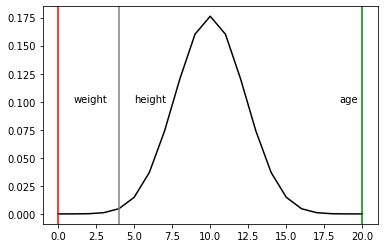
Let's take a feature (no matter if age, height or weight) and say we have absolutely no clue if it's useful or not. What is the probability that we shall keep it? The level of uncertainty about the feature is expressed by a probability of 50%, like tossing a coin. Since each independent experiment can give a binary outcome (hit or no hit), a series of n trials follows a binomial distribution.
In Python, the probability mass function of a binomial distribution can be computed as follows:
import scipy as sp

trials = 20
pmf = [sp.stats.binom.pmf(x, trials, .5) for x in range(trials + 1)]
print(pmf)

# plot the probability mass function pyplot.plot(list(range(0,trials+1)), pmf, color = "black")
pyplot.axvline(hits_df.loc[hits_df['var'] == 'age','total hits in iteration'].values, color = 'green')
pyplot.text(hits_df.loc[hits_df['var'] == 'age','total hits in iteration'].values -1.5,.1, 'age')
pyplot.axvline(hits_df.loc[hits_df['var'] == 'weight', 'total hits in iteration'].values, color = 'red')
pyplot.text(hits_df.loc[hits_df['var'] == 'weight', 'total hits in iteration'].values + 1, .1, 'weight')
pyplot.axvline(hits_df.loc[hits_df['var'] == 'height', 'total hits in iteration'].values, color = 'gray')
pyplot.text(hits_df.loc[hits_df['var'] == 'height', 'total hits in iteration'].values + 1, .1, 'height')
pyplot.show()

The values above look like a bell curve.
In Boruta, there is not a hard threshold between a refusal and an acceptance area.
Instead, there are three areas:
an area of refusal (the left tail): the feature that ends up here are considered as noise, so they are dropped;
an area of irresolution (center): the Boruta is indecisive about the features that are in this area;
an area of acceptance (the right tail): the features that are here are considered as predictive, so they are kept.
The areas are defined by selecting the two most extreme portions of the distribution called tails of the distribution.
So, we did 20 iterations on our data and ended up with some statistically grounded conclusions:
in order to predict the income of a person, age is predictive and should be kept, weight is just noise and should be dropped,
Boruta was indecisive about height: the choice is up to us, but in a conservative frame, it is advisable to keep it.
In the next section we will introduce BorutaPy in Python.
Installing and running Boruta
The Boruta Python package can be installed via pip:
pip install borutaOnce installed, we will want to import BorutaPy and execute Boruta as shown below:
from boruta import BorutaPy
from sklearn.ensemble import RandomForestRegressor
import numpy as np

### setup Boruta
forest = RandomForestRegressor(n_jobs = -1, max_depth = 5)

boruta = BorutaPy(
estimator = forest,
n_estimators = 'auto',
max_iter = 50 # number of trials to perform
)

### fit Boruta (it accepts np.array, not pd.DataFrame)
boruta.fit(np.array(X), np.array(y))

### print results
accepted = X.columns[boruta.support_].to_list()
print('Accepted features:', accepted)
> Accepted features: []

undecided = X.columns[boruta.support_weak_].to_list()
print('Undecided features', undecided)
> Undecided features ['age']

selected_features = accepted + undecided # include undecided for safe measure
print(selected_features)
> ['age']
And there you have it! Note that we ran 50 trials in the above example whereas we had previously ran 20 trials in our longhand example, which is why age was initially considered 'accepted' and this run it was considered 'undecided'. However, we still land with age being a selected feature to predicting income after combining our accepted and undecided features.
In summary
As mentioned in the beginning, I've found great success using the Boruta package in R to quickly select top predictors in my feature selection efforts. The approach is clever but yet simplistic!
I hope you found this to be a worthwhile read. Feel free to message me if you have questions or have found success with other feature selection approaches. Happy feature hunting!

Comments